Effects on the Economy: Does it Matter Which Political Party is in Power?

In light of the United State's current economic condition, one should consider how voting for a particular party affects the overall state of the country's economy. Republicans and Democrats both accuse the opposing party of causing economic downturns. Republicans argue that the Democrats' increased government spending and regulation of industry stifles the economy. On the other hand, Democrats argue that the Republicans goal to deregulate private industry encourages businesses to take dangerous risks that could potentially harm the nation's economy as a whole.

So which party has it right? Under the leadership of which party does the U.S.'s economy thrive or decline?

Using a data set from the Bureau of Economic Analysis (BEA), I was able to compile a list of both the annual and quarterly change in GDP since 1930. I then created a variable for the President's party for every year in the data set (1 for a Democratic president and a 2 for a Republican president).

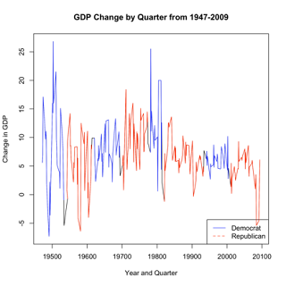
I then began comparing the change in GDP under Democratic Presidents to the change in GDP under Republican Presidents. The first figure tracks the change in GDP in each quarter from 1947 to 2009. When the line is blue, a Democratic president was in office and when the line is red, a Republican president was in office.

This figure is simply a time line of GDP growth and decline and fails to help answer the question. One simply cannot tell if there is more growth under Democratic leadership or under Republican.

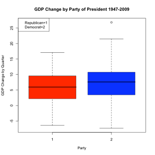
The second figure presents a boxplot that compares the GDP quarterly change under Republican Presidents (red) versus Democratic Presidents (blue).

What is revealed in the boxplot is that under Democratic leadership there is a slightly larger mean GDP growth. This means that under a Democratic president there is slightly more growth in GDP. Also, the upper-quartile of the Democratic (blue) boxplot is greater than the upper-quartile of the Republican (red) boxplot. This means that the greatest growth in GDP since 1947 was experienced under the leadership of a Democratic president. Although both of these findings are intriguing, they are hardly evidence that the economy fairs better under Democratic leadership.

The third figure is a collection of scatterplots. Each scatterplot represents a sequence of time when the country was under either Democratic or Republican leadership. I plotted GDP quarterly change over time and added a reference line to help the viewer see whether there was either GDP growth or decline. The blue plots represent a length of time when a Democrat was president and the red plots represent a length of time when a Republican was president.

The main observation from these sequence of plots is that there is an equal amount of growth and decline under Democratic and Republican presidents. From the plots, it appears that when there is decline under a Democratic president, it is followed by a period of decline under a Republican president. When there is growth under a Democratic president, it is followed by a period of growth under a Republican president. This pattern is found in all but the last two plots. In the 1994-2001 plot (Bill Clinton-Democrat), GDP growth was detected. However, this period of growth under a democratic president was followed by a period of GDP decline from 2002-2009 under a republican president (George W. Bush). Overall, this sequence of plots is informative and it suggests that the economy fairs equally well under the leadership of either party.

In the fourth figure, I compare the distribution of GDP change under Democratic presidents (blue) to the distribution of GDP change under Republican presidents (red).

What is most obvious from these two histograms is that the distribution of GDP change under either Democratic or Republican presidential leadership appears to be essentially the same. Both distributions are centered around 5 percent GDP growth. Both distributions have cases of extreme GDP growth and decline. Of course, looking at distributions presented in histograms can be misleading, because the number of bins can change the appearance of the distribution drastically.

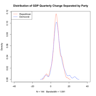
In order to better compare the two distributions, I created a fifth figure that plots the kernel density distribution for GDP Quarterly change under both Republican and Democratic presidencies. The blue line represents the distribution under Democratic leadership and the red line represents the distribution under Republican leadership.

What is most immediately obvious is that the distribution of GDP quarterly change under either democratic or republican presidents is the same. In fact, the two distributions are almost identical. The main differences are that under Republican presidencies there are more cases of the mean growth. Also, the democratic distribution has more cases of extreme growth, which can be observed in its upper tail. This, however, does not serve as evidence that the country does better under Democratic rule. Other than those two differences the distributions are pretty much the same.

These visualizations suggest that the party that controls the executive branch does not determine whether the U.S. economy will thrive or decline. Under the leadership of both parties the economy experienced times of growth and times of decline.

Link to data: http://www.bea.gov/national/index.htm

R Code:

##Loading Data

econ<-read.csv("/Users/carrielevan/Documents/Geo299/EconomicHW/GDPchange.csv")

library(car)

NOTE: For some reason my code under "preparing the data" keeps changing once I post. I've tried it three times and don't know why it changes. If you want the exact code, email me and I will give it to you.

##Preparing the Data

#Subsets of GDP Quarter Change by Party in Power

dem1<-subset(econ$GDPQuarterChange, econ$Quarter<>

rep1<-subset(econ$GDPQuarterChange, econ$Quarter>19534 & econ$Quarter <>

dem2<-subset(econ$GDPQuarterChange, econ$Quarter>19614 & econ$Quarter <>

rep2<-subset(econ$GDPQuarterChange, econ$Quarter>19694 & econ$Quarter <>

dem3<-subset(econ$GDPQuarterChange, econ$Quarter>19774 & econ$Quarter <>

rep3<-subset(econ$GDPQuarterChange, econ$Quarter>19814 & econ$Quarter <>

dem4<-subset(econ$GDPQuarterChange, econ$Quarter>19814 & econ$Quarter <>

rep4<-subset(econ$GDPQuarterChange, econ$Quarter>19934 & econ$Quarter <>

dem4<-subset(econ$GDPQuarterChange, econ$Quarter>19934 & econ$Quarter <>

rep4<-subset(econ$GDPQuarterChange, econ$Quarter > 20004)

#Creating Subset of Quarter Dates

demQ1<-subset(econ$Quarter, econ$Quarter <>

repQ1<-subset(econ$Quarter, econ$Quarter>19534 & econ$Quarter <>

demQ2<-subset(econ$Quarter, econ$Quarter>19614 & econ$Quarter <>

repQ2<-subset(econ$Quarter, econ$Quarter>19694 & econ$Quarter <>

demQ3<-subset(econ$Quarter, econ$Quarter>19774 & econ$Quarter <>

repQ3<-subset(econ$Quarter, econ$Quarter>19814 & econ$Quarter <>

demQ4<-subset(econ$Quarter, econ$Quarter>19934 & econ$Quarter <>

repQ4<-subset(econ$Quarter, econ$Quarter > 20004)

##FIgure 1

#Line Plot with Different Party in Power lines

plot(econ$Quarter, econ$GDPQuarterChange, xlab="Year and Quarter", ylab="Change in GDP", main="GDP Change by Quarter from 1947-2009", type="l")

lines(demQ3, dem3, col="blue")

lines(demQ4, dem4, col="blue")

lines(demQ2, dem2, col="blue")

lines(demQ1, dem1, col="blue")

lines(repQ2, rep2, col="red")

lines(repQ1, rep1, col="red")

lines(repQ3, rep3, col="red")

lines(repQ4, rep4, col="red")

legend("bottomright", c("Democrat", "Republican"), col=c("blue", "red"), lty=1:2)

##Figure 2

#Boxplot

boxplot(GDPQuarterChange~PID, data=econ, ylab="GDP Change by Quarter", xlab="Party", main="GDP Change by Party of President 1947-2009", col=(c("red", "blue")))

legend("topleft", c("Republican=1", "Democrat=2"))

##Figure 3

#Plots on One Image

par(mfrow=c(2,2))

plot(demQ1, dem1, type="p", xlab="Year and Quarter", ylab="GDP Change by Quarter", main="GDP Change under Democratic President 1947-1953", col="blue")

abline(lm(dem1~demQ1), col="blue")

plot(repQ1, rep1, type="p", xlab="Year and Quarter", ylab="GDP Change by Quarter", main="GDP Change under Republican President 1954-1961", col="red") abline(lm(rep1~repQ1), col="red")

plot(demQ2, dem2, type="p", xlab="Year and Quarter", ylab="GDP Change by Quarter", main="GDP Change under Democratic President 1962-1969", col="blue")

abline(lm(dem2~demQ2), col="blue")

plot(repQ2, rep2, type="p", xlab="Year and Quarter", ylab="GDP Change by Quarter", main="GDP Change under Republican President 1970-1977", col="red")

abline(lm(rep2~repQ2), col="red")

par(mfrow=c(2,2))

plot(demQ3, dem3, type="p", xlab="Year and Quarter", ylab="GDP Change by Quarter", main="GDP Change under Democratic President 1978-1981", col="blue")

abline(lm(dem3~demQ3), col="blue")

plot(repQ3, rep3, type="p", xlab="Year and Quarter", ylab="GDP Change by Quarter", main="GDP Change under Republican President 1982-1993", col="red")

abline(lm(rep3~repQ3), col="red")

plot(demQ4, dem4, type="p", xlab="Year and Quarter", ylab="GDP Change by Quarter", main="GDP Change under Democratic President 1994-2001", col="blue")

abline(lm(dem4~demQ4), col="blue")

plot(repQ4, rep4, type="p", xlab="Year and Quarter", ylab="GDP Change by Quarter", main="GDP Change under Republican President 2002-2009", col="red")

abline(lm(rep4~repQ4), col="red")

##Figure 4

#Preparing the Data

REP1<-subset(econ$GDPQuarterChange, econ$QuarterPID==1)

DEM1<-subset(econ$GDPQuarterChange, econ$QuarterPID==2)

dREP1<-density(REP1)

dDEM1<-density(DEM1)

#histogram

par(mfrow=c(2,1))

hist(DEM1, col="blue", main="Histogram of GDP Quarterly Change Under Democratic President", xlab="GDP Quarterly Change", breaks=15)

hist(REP1, col="red", main="Histogram of GDP Quarterly Change Under Republican President", xlab="GDP Quarterly Change", breaks=15)

##Figure 5

plot(dREP1, main="Distribution of GDP Quarterly Change Separated by Party", col="red", xlim=c(-40,40))

lines(dDEM1, col="blue")

legend("topleft", c("Republican", "Democrat"), col=c("red", "blue"), lty=1:1)

A Replication: Hockey Stick Visualization

Review: The Hockey Stick Controversy, Still Heated

When Michael Mann, Raymond Bradley and Malcolm Hughes first presented their findings that suggested the globe’s warming was greater than had been experienced in the past, they never would have predicted that one simple graphic would alter domestic and international politics for decades to come. Mann et al. had unintentionally created the “hockey stick controversy.” In their 1998 paper, Mann et al. were interested in investigating the three following questions: Was the globe warming; If so, was the warming within normal patterns of past warming; Finally, if the globe was warming and the warming was not within the trend of past warming periods, was it caused by humans?

In order to investigate these questions, Mann et al. used two different types of measurement methods. The first type is what I call “controversial measurements.” These are measurements taken using tree rings, corals, ice cores, and other historical records to estimate the earth’s past temperatures. Since these measurements are estimates of unknown past temperatures, the accuracy of the data is questioned, which is why they are deemed “controversial.” Furthermore, those who oppose the claim that the earth is warming reference their dissatisfaction and skepticism of these measurements to support their side of the global warming debate.

The second type used in Mann’s study was what I call “thermometer measurements.” As the name suggests, these measurements are thermometer records of the earth’s temperature. They are more contemporary and considered accurate measurements. These data have been collected since 1902 and continue to be collected and recorded today. By combining the two types of data collected, Mann et al. were able to track the earth’s temperature records back until 1400 (in the data set I used) and in later versions of the paper as early as 1000 AD. This allowed the team of researchers to compare the earth’s temperatures in the past to the earth’s temperature of the present and begin to answer their first question.

Their first question of interest was whether or not the globe was in fact warming. Mann et al. did find evidence that suggested that the earth was warming. Once coming to this conclusion, the team moved onto their second question: was this pattern of warming outside of the normal ebb and flows of global warming and cooling? Mann and his team argued that the data suggested that the contemporary pattern of warming was outside the normal trend. After this conclusion, the group of researchers moved onto their final question, which was: Is global warming caused by humans? After much analysis, Mann et al. determined that it was manmade.

In order to present their findings, the team put together a graphic that illustrated the global warming pattern they believed the data revealed. The graphic they created is what is known today as “The Hockey Stick Graph.” The graph reveals that from 1400 AD until about 1900 the earth’s temperature was relatively consistent. In the graph, this period of time is represented by an essentially flat or steady line and creates the “shaft” of the hockey stick. Around 1900, the earth’s temperature began to rise steadily and continues to increase today. This rise in temperature is represented in the graph by a climbing line and this line creates the blade of the hockey stick.

The graphic alone reveals Mann’s answers to his three questions. It clearly illustrates that the earth’s temperature was and is rising. It also suggests that this increase is greater than the normal heat waves the earth had experienced in the past. This is evident when one compares the increases found in early time periods (the blue line), which were measured using the controversial methods, to the increases found since 1900 (the red line), which are measurements taken using the thermometer method. Once the red line hits the 1990’s, record temperatures were being documented. In no previous period presented on the graph were temperatures of equal magnitude being found. This suggests that the current heating of the earth is some how different from earlier periods. Finally, the graph also suggests that this pattern of abnormal global warming was and continues to be caused by humans. An observer of the graph can see that the earth’s rising temperatures began around 1900. This, of course, is towards the end of the Industrial Revolution, a time period of massive manufacturing, transportation, and mining transformation. More importantly, it was a time period when humans had begun burning fossil fuels. The fact that the peak of the Industrial Revolution coincides with the rise in the earth’s temperatures suggests that the two may be related. If this is the case, then it serves as evidence that global warming is caused by humans.

Despite the initial clarity of the graph, many global warming critics accuse the use of the graphic as misleading. These critics, as previously mentioned, are extremely skeptical of the use of the “controversial measurements” of the Earth’s past temperatures. They argue that the uncertainty in these measurements, when ignored, lead observers of the analysis with a sense that the findings are conclusive and absolute.

In response to the critique that the graph is misleading, however, I argue that Mann et al. were very open and honest with their data. After all, within the hockey stick graph, they reveal the standard errors for the controversial measurements. The gray shaded area behind the blue line is the standard error and any informed reader of the graph would understand that this shaded area represents the level of uncertainty present in the data. In other words, the earth’s “true” past temperature is estimated to be within the shaded area. So, the past temperature may be greater than what the blue line suggests, which would mean that the contemporary warming of the globe is not exceptional. And the Earth’s past temperature may also be less than what the blue line suggests, which would mean the current heating of the earth is more severe than originally believed to be. Had Mann and his fellow researchers excluded the presentation of the standard errors altogether, I would have agreed with their critics that the graph was misleading. However, Mann did present the standard errors and so this criticism is not justified.

In response to the claim that the “controversial measurements” cannot support the conclusion that the globe is in a current state of warming that differs from previous periods of warming because the measurements are inaccurate depictions of past temperatures, I argue that there is a simple way to show how accurate or inaccurate these measurements are. Starting in 1902, there is data collected using both methods (the controversial and thermometer methods). By comparing the measurements taken using both methods, one can see if they produce the same results. I did this very test in my extension and what I found was that both methods measured the earth’s temperature at essentially the same level (look at my second graph under extension). This test also discredits global warming critics’ claim that the data used to measure past temperatures are inaccurate.

Of course, my simple test does not come anywhere near closing this debate. In fact, the continuous research and repeated findings that corroborate with Mann’s initial findings over the last 20 years have not put the controversy to rest. Despite this continuous research and repeated findings, global warming critics continue to find any mistake, or misuse of the data to argue that “climate change” is nothing but a hoax. These critics’ claims are not without ground, especially in light of the recent IPCC report mistake, which accidentally claimed that the Himalayan Glaciers would disappear in 2035 as opposed to 2350. Incidents like these give fuel to critic’s fire. Furthermore, critics use these few mistakes to completely discount the thousands of valid studies that do support Mann’s initial findings.

Currently, the debate between the two sides is extremely political at both the domestic and international level and the fighting between the two sides only seems to get more “heated.” Of course, hot tempers may simply be a side effect to climate change.

Replication of Mann et. Al 1998 Hockey Stick Graphic

I used the data from Mann et. al. 1999 paper. This data contains temperature measurements from the year 1400 and continues until the year 1995. The following image is my replication of Mann's 1999 graphic:

I used the following code in R to produce the visualization:

#Loading Data

load("/Users/carrielevan/Downloads/hockey.rdata")

#Creating Line for Thermometer Measurements (Contemporary Measurements)

plot(hockey$date, hockey$raw, type="l", col="red", ylim=c(-1.1, 0.8), ylab="Departures in temperature (C)\ from the 1961 to 1990 average", xlab="Year", main="Northern Hemisphere")

#Creating SE Shaded Region

polygon(x=c(hockey$date, rev(hockey$date)), y=c(hockey$sigpos1, rev(hockey$sigpos2)), col="gray83", border=FALSE)

#Creating Tree Rings, Corals, Ice Cores, and Historical Records Line

lines(hockey$date, hockey$recon, col="dodgerblue3")

#Creating Trend Line

meanRAW<-mean(hockey$raw)

abline(h=meanRAW)

#Creating Lowess Line

lowess<-lowess(hockey$date, hockey$recon, f=0.04, iter=3)

lines(lowess)

Extension of Mann's Analysis

Many of Mann's critics argue that his use of data gathered from tree rings, corals, ice cores, and historical records are inaccurate and so exaggerate the claim that the globe is warming. In order to further investigate this criticism, I will compare the "controversial measurements" (temperature measurements taken from tree rings, corals, etc.) with the contemporary measurements taken with thermometers.

Starting in 1902, there is data available for both the "controversial measurements" and the "thermometer measurements." Since there is overlap, I am able to compare the two measurements and through this comparison, I will be able to show whether or not the two methods for measuring the globe's temperature differ greatly or not at all.

In the first graph, I compare the two measurements over the entire span of time available in the data (1400-1995). One can see that around 1900, the "thermometer measurements" (the red line) and the "controversial measurements" (the blue line) almost perfectly match. This is true until about 1980, when the two lines diverge and appear to be moving in the opposite directions. Of course, this is a startling finding, because Mann claims that in the 90's the greatest global temperature increases occurred. The finding, however, that the thermometer measurements and the controversial measurements no longer match after 1980 seems to injure the validity of Mann's conclusions.

In order to further investigate this pattern, I isolated the time period between 1900 and 1995. In the second graph, one can observe how the two measurements follow each other almost exactly. Furthermore, the supposed differentiation between thermometer and controversial measurements found in the first graph, in the second graph, is found to be simply a lack of "controversial measurements" taken. In fact, between 1980 and 1995 no "controversial measurements" are available. So, upon closer inspection, one can see that the criticism that these "controversial measurements" are inaccurate measurements of past temperatures does not seem to hold, at least for the time period between 1902 and 1980. Both thermometer and controversial measurements of temperature produce essentially the same data.

R Code for Extension

#Comparison Between two Temperature Measurement

#Erasing the Zero Values

recon1<-hockey$recon

hockey$recon1<-recon1

fix(hockey)

hockey$recon1[hockey$recon1==0]<-NA

#Creating the Lowess Lines

lowessRAW1<-lowess(hockey$date, raw1, f=0.04, iter=3)

lowessRECON1<-lowess(hockey$date, recon1, f=0.04, iter=3)

#Creating Plot 1

plot(lowessRAW1, type="l", col="red", ylim=c(-0.5, 0.8), xlim=c(1400, 2000), main="Comparison of Thermometer Measurements\n and Controversial Measurements\n (lowess smoother)", xlab="Year", ylab="Difference in Temperature (C) from 1400-1995")

lines(lowessRECON1, type="l", col="blue")

abline(h=meanRAW)

legend("bottomright", c("Thermometer", "Controversial"), col=c("red", "blue"), lty=1:2)

######Now to Isolate effects between 1902 and 1995

#Creating a Subset of the data for only 1902 and Later

raw2<-subset(hockey$raw, hockey$date>1902)

date2<-subset(hockey$date, hockey$date>1902)

recon2<-subset(hockey$recon, hockey$date>1902)

#Creating Plot 2

plot(date2, raw2, type="l", col="red", main="Closer Look: Comparison of Thermometer Measurements\n and Controversial Measurements", xlab="Year", ylab="Difference in Temperature (C) from 1902 to 1995")

lines(date2, recon2, type="l", col="blue")

legend("bottomright", c("Thermometer", "Controversial"), col=c("red", "blue"), lty=1:2)

Visualizations in The Study of American Voting Behavior

In the field of American voting behavior, the use of creative visualizations is an untapped resource. Rarely do researchers use innovative images to help tell their story. Instead, researchers in this field tend to rely on traditional visualizations like scatter plots and histograms. The three sets of images presented here help illustrate a few examples of how researchers of American voting behavior have used innovative visualizations to help inform their viewers.

The first collection of maps, “2008 Presidential Election Results,” uses visualizations to tell a very compelling story. Mark Newman shows how the traditional election results map, simply cast in red if the majority of a state’s population voted for the Republican candidate and blue if the majority of a state’s population voted for the Democratic candidate, is misleading.He argues that by not taking into consideration the distribution of population, the map appears that the Republican candidate should have won the election. Using a cartogram to rescale the size of a state according to its population, the rescaled election results map tells a completely different story. Newman also uses a cartogram at the county level to reveal, once again, how the traditional results map is misleading. This collection of visualizations is extremely useful, because they help tell a story that words alone would not sufficiently describe. The images reveal information in a clear and concise manner and without even reading the article, observers would understand Newman’s argument.

The second set of maps, however, are not extremely useful. In their article “The Republicans Should Pray for Rain: Weather, Turnout, and Voting in U.S. Presidential Elections,” Gomez, Hansford, and Krause argue that rain on Election Day depresses turnout, which then helps Republican candidates win elections. The only images they use to help tell their story are two maps of the United States. In the first map, they show the distribution of precipitation on the Election Day with the least amount of rain. In the second map, they show the distribution of precipitation on the Election Day with the most rain. These two images are not particularly informative, because they are not providing the reader with any insight that they could not have received without images. Furthermore, the images fail to connect turnout to rainfall, which is the very relationship the authors are interested in investigating.

The final map illustrates the distribution of access to the Fox News Network in 2000.Researchers Della Vigna and Kaplan are interested in investigating the effects of the entry of Fox News Network into the cable news line-up on voting behavior. They find that the Fox News Network “convinced” 3 to 28 percent of their viewers to vote for a Republican candidate. They use the map to illustrate which voters had access to the news network at the time of the 2000 General Presidential election. The map is useful, because it reveals which citizens had the option to watch Fox News, which then helps the viewer understand the demographics of the channel’s potential viewership. However, without the content of the article the image is not incredibly informative and doesn’t reveal the connection between vote decision and access to the network on its own.

Voting behavior specialists have underutilized innovative visualizations. Instead, they turn to traditional images like scatter plots, which were not displayed in this small collection of images, to help tell their stories. Although these traditional forms of visualizations are useful and informative, the potential for more creative visualizations has been underused. New technology and access to massive amounts of rich data allows researchers to tell their stories through informative, creative and easily readable images.

2008 Presidential Election Results

The following maps present the 2008 Presidential election results at both the state and county level. Most of you have seen the traditional mapping of the presidential election results where states whose population voted a majority Republican are painted red and states whose population voted a majority Democrat are painted blue.

This particular researcher adds a twist to these very common maps by taking into account the population size of the state or county. Mark Newman argues that the traditional maps are misleading because they do not account for each state or county's population size. In order to account for this discrepency, Newman makes cartograms of the election results at both the state and county level. These cartograms rescale the states or counties based on the size of their population. In other words, states with large populations appear geographically larger and vice versa.

By rescaling the states and counties by population size, viewers get a more accurate depiction of the distribution of votes for the 2008 Presidential Election.

Link to article: http://www-personal.umich.edu/~mejn/election/2008

Effects of Rain on Voter Turnout and Election Results

In the next article, Gomez, Hansford, and Krause are trying to illustrate the effects that weather has on voter turnout and election results. The argue that rainy weather depresses turnout and also helps Republican candidates.

The map posted below shows the distribution of rain on election day for elections with the least amount of rain and the most rain.

Link to article: http://myweb.fsu.edu/bgomez/GomezHansfordKrause_JOP_2007.pdf

Effects of Fox News Network on Vote Choice in the 2000 Presidential Election

In the third article, Della Vigna and Kaplan argue that the establishment of the Fox News Network impacted voting in 2000. They found that the Fox News Network "convinced" 3 to 28 percent of their viewers to vote Republican in 2000.

The following map illustrates the distribution of access to the Fox News Network in 2000.

Link to article: http://elsa.berkeley.edu/~sdellavi/wp/foxvote06-03-30.pdf